Synergy2 is a reimplementation of Synergy, originally developed at The Broad Institute and described by Wapinski et al in Nature and Bioinformatics. This software resolves ortholog clusters by leveraging both homology and synteny in the context of a species tree. It is applicable to both prokaryotic and eukaryotic data sets of variable diversity.
1. Downloading and Installing Synergy2
Download the latest version of Synergy2 from Sourceforge.
1.1. Dependencies
Synergy2 has several package dependencies, all of which are available below.
1.1.1. Hardware
Synergy2 is designed to run on a distributed grid environment. Synergy2 can also be run locally on a multi-core machine. The results will be identical for both serial and parallel executions.
1.2. Installation
After all dependencies have been satisfied, run INSTALL.py. When prompted for paths to executables, provide the complete path.
2. Running Synergy2
Synergy2 is executed in 3 steps:
-
Satisfy data dependencies
-
Genome sequences
-
Genome annotations
-
Species tree
-
-
Initialization
-
Data preparation
-
Taxa relationship definition
-
Parameter definition
-
-
Computation
2.1. Data Dependencies
For each genome to be analyzed, Synergy2 requires the genome sequence and structural gene annotation. A species tree must define the relationship between all genomes. A data catalog tracks the location of these data.
2.1.1. Genome Sequence
The genome sequence must be in FASTA format. The sequence headers must correspond to those in the structural annotation file.
2.1.2. Structural Gene Annotation
Structural annotations are described in GFF3 format. The data in the first column must correspond to the headers in the genome sequence file. Gene structure elements (3rd column) of "gene" and "exon" are required. The 9th column must contain "ID=<string>", where <string> is a unique identifier of that particular gene. Names,locus tags and other descriptors from this column will be ignored.
7000000186464702        EntFae_Aus0004_GB1      gene    262137  263042  .       +       .       ID=7352927015;Name=hypothetical protein
7000000186464702        EntFae_Aus0004_GB1      mRNA    262137  263042  .       +       .       ID=7352927016;Parent=7352927015
7000000186464702        EntFae_Aus0004_GB1      exon    262137  263042  .       +       .       ID=7352927018;Parent=7352927016
7000000186464702        EntFae_Aus0004_GB1      CDS     262137  263042  .       +       .       ID=cds7352927016;Parent=7352927
2.1.3. Data Catalog
A file containing the complete path to the genome sequence and corresponding structural gene annotation in must be provided.
//
Genome Bsub_E342_V1
Sequence /path/to/Bsub_E342_V1_sequence.fa
Assembly /path/to/Bsub_E342_V1_annot.gff3
//
Genome EntFae_Aus0004
Sequence /path/to/EntFae_Aus0004_sequence.fa
Assembly /path/to/EntFae_Aus0004_annot.gff3
//
2.1.4. Species Tree
The tree must be unrooted and in Newick format. Branch lengths may be in decimal or scientific notation. Bootstrap values, while allowed, will not factor into the algorithm. If the tree has ancestral nodes with more than two children, the children will be randomly grouped into pairs.
|
|
If the resolution of the initial species tree is unsatisfactory, a new species tree can be generated from the single copy core after Synergy2 has been run. At that point, Synergy2 may be re-run with the updated tree. Computations will only be performed where the topology has changed. |
2.1.5. Using AMPHORA2 to create a species tree
If no species tree is available, the user can create a species tree based on 39 protein HMMs defined by AMPHORA2.
2.2. Initialization
After all of the data requirements have been satisfied, the user runs WF_runSynergy2.py. This script defines the WorkFlow instance and creates all of the dependent files. This is also the control point for the user to define various parameters.
2.2.1. Computational Resource Variables
These variables impact the run-time performance of Synergy2.
BLAST - # of cores, default=4: This is configured during install, but can be modified here.
Wait for File - update frequency, default=60s: How often, in seconds, a sub workflow checks to see if its dependencies have been satisfied. Generally should not be changed.
2.2.2. Algorithmic Variables
These variables impact the output of Synergy2.
Rough Clusters
Blast e-value, default=0.01: Determines the minimum quality of acceptable hit. Only best hits will be considered to define rough clusters, but all hits will be used to compute syntenic fractions and distance matrices. Consequently, this cut-off is not stringent.
Syntenic window size, default=5kb: Extends to the left and right of the gene in question. A 5kb window evaluates a total of 10kb surrounding each gene. Raise or lower based on the assumed range of syntenic conservation in your analysis.
Minimum "Best Hit" score, default=0.5: This determines the tightness of the rough clusters. A lower value creates larger rough clusters as it allows for more variation, while a higher value does the opposite. This score is representative of the quality and coverage of the hit. The coverage is calculated with respect the percent identity and query vs target coverage of the hit.
Scaling of contribution for graph edges, default homology=0.01, default synteny=1.0: Impacts the weight of homology (BLAST) and synteny when a cluster’s gene tree is rooted or evaluated. Because homology is used to create the partitions for the gene tree, it is scaled back. If the genomes are particularly fragmented, homology weight may be increased to allow for differentiation.
Tree Rooting
gamma, default=10.0
A factor in the gene tree rooting equation that affects the impact of gain and loss events
gain, default=0.05
The probability of a gain event at a given ancestral node
loss, default=0.05
The probability of a loss event at a given ancestral node
2.3. Computation
2.3.1. Running the WorkFlow instance
WF_runSynergy2.py returns a list of commands that need to be executed in order to set up the working environment. These commands, found in genomes/needed_extractions.cmd.txt, can be run serially or distributed to a grid. After the working environment has been set up, re-run WF_runSynergy2.py the same as before. This will create a [flow].xml and a [flow].ini file in your Synergy2 working directory, where [flow] is defined by -f or --flow. You are now ready to run the actual algorithm.
Set up the command line environment.
source /path/to/workflow/exec_env.tcsh
use LSF (make sure your grid distribution module is loaded)
Launch instance_commands.txt to the grid. If you have queues for different time periods, an average Synergy2 run of 150 E.coli genomes can be completed in about 12 hours across 50 nodes.
Then, the WorkFlow instance may be dispatched as follows:
RunWorkflow -t [flow].xml -c [flow].ini -i [instance].xml &
This is not necessary for the execution of Synergy2, but will allow you to monitor its progress.
3. Example Data Set
The files in this data set are in the Synergy2 distribution in example/.
This is a simple example using 5 E.coli genomes. Their relationships are defined by an unrooted species tree.
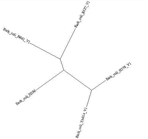
((Esch_coli_H378_V1:0.001,Esch_coli_TA014_V1:0.0014):0.002,((Esch_coli_H461_V1:0.0012,Esch_coli_R527_V1:0.001):0.0015,Esch_coli_H296:0.003):0.0025);3.1. Preparing the Data
The following steps will generate ortholog clusters as well as a validation method to ensure that your installation of Synergy2 is functioning correctly.
Make your current working directory (CWD) example/, and get the complete path of your CWD.
Synergy2 $ cd example/
example $ pwd
/home/utilities/Synergy2/example/
Edit data_catalog.txt to reflect the complete path to each file
//
Genome  Esch_coli_H296
Sequence        /home/utilities/Synergy2/example/Esch_coli_H296/Esch_coli_H296.genome
Annotation      /home/utilities/Synergy2/example/Esch_coli_H296/Esch_coli_H296_PRODIGAL_2.annotation.gff3
//
Genome  Esch_coli_H378_V1
Sequence        /home/utilities/Synergy2/example/Esch_coli_H378_V1/Esch_coli_H378_V1.genome
Annotation      /home/utilities/Synergy2/example/Esch_coli_H378_V1/Esch_coli_H378_V1_PRODIGAL_2.annotation.gff3
//|
|
A species tree has been provided for this example (example/tree.nwk). It is unrooted and in newick format. A tree is required for Synergy2. If, for other data sets, a species tree does not exist, one can be constructed with AMPHORA2. |
Create a working directory for this clustering analysis and move into it.
example $ mkdir test
example $ cd test/
At this point, all data dependencies have been satisfied and the Synergy2 working directory can be populated with data. For this example, the default values are used. To see the current defaults:
test $ ../../bin/WF_runSynergy2.py --help

        python WF_runSynergy2.py [OPTIONS]

        -h, --help
                Prints this usage and exits
        REQUIRED:
        -r, --repo [file]
                where [file] is the complete path to the data repository containing your genomic data
        -w, --working [path]
                where [path] is the complete path to the working directory for this analysis
        -t, --tree [file]
                where [file] is a species tree relating all of the genomes to be analyzed
        -f, --flow [string]
                where [string] is any string you choose, and will be the template of your Workflow instance

        OPTIONAL ALGORITHM VARIABLES:
        -g, --gamma [float]
                where [float] is a factor in the rooting equation, default = 10.0
        -G, --gain [float]
                where [float] is the probability of a gain event occurring, range (0.0, 1.0], default = 0.05
        -L, --loss [float]
                where [float] is the probability of a loss event occurring, range (0.0, 1.0], default = 0.05
        -b, --blast_eval [float]
                where [float] is the e-value used for all blast analysis, default = 0.01
        -m, --min_best_hit [float]
                where [float] is the minimum score a blast hit must have to define an edge in the initial clusters, range (0.0, 1.0], default = 0.5
        -s, --synteny_window [int]
                where [int] is the distance in base pairs that will contribute to upstream and downstream to syntenic fraction.  The total window
                size is [int]*2. default = 5000
        -S, --synteny_scale [float]
                where [float] represents the contribution of synteny to branch weight for cluster trees, range (0.0, 1.0], default = 1.0
        -H, --homology_scale [float]
                where [float] represents the contribution of homology to branch weight for cluster trees, range (0.0, 1.0], default = 0.01
        -T, --top_hits [int]
                where [int] is the number of blast hits that will be considered for each gene, default=5
        -l, --locus [file]
                where [file] is a locus_tag_file.txt that corresponds to the data in this repository
        -D, --hamming [float]
                where [float] is the maximum hamming distance between a representative sequence and a sequence being represented
                range [0.0,1.0], default=0.6

        OPTIONAL PERFORMANCE VARIABLES:
        -n, --num_cores [int]
                where [int] is the number of cores used for blast analysis (-a flag), default = 6
3.2. Run Synergy2
Populate the data structures and create the Workflow files by running WF_runSynergy2.py from test/
test $ ../../bin/WF_runSynergy2.py -r /home/utilities/Synergy2/example/data_catalog.txt
-w /home/utilities/Synergy2/example/test/ -t /home/utilities/Synergy2/example/tree.nwk -f test_flow
Wrote locus tags to locus_tag_file.txt
Launch this command file on the grid: /home/utilities/Synergy2/example/test/genomes/needed_extractions.cmd.txt
Run the commands in genomes/needed_extractions. After all commands have finished, re-run the WF_runSynergy2.py command exactly as before
test $ ../../bin/WF_runSynergy2.py -r /home/utilities/Synergy2/example/data_catalog.txt
-w /home/utilities/Synergy2/example/test/ -t /home/utilities/Synergy2/example/tree.nwk -f test_flow
Wrote locus tags to locus_tag_file.txt
init tree lib
reading genome to locus
reading tree
((Esch_coli_H378_V1:0.001,Esch_coli_TA014_V1:0.0014):0.002,((Esch_coli_H461_V1:0.0012,Esch_coli_R527_V1:0.001):0.0015,Esch_coli_H296:0.003):0.0025);
parsing tree
VDY;ZGN XSL
IBX;OXY IGQ
IGQ;SVM HAY
XSL:0.002,HAY:0.0025
rooting
('XSL', 'HAY')
XSL 2 [('XSL', 'VDY'), ('XSL', 'ZGN')]
edge from root to XSL
XSL 3 {'VDY': {'weight': 0.0014}, 'root': {'weight': 0.001}, 'ZGN': {'weight': 0.001}}
HAY 2 [('HAY', 'SVM'), ('HAY', 'IGQ')]
edge from root to HAY
HAY 3 {'SVM': {'weight': 0.0030000000000000001}, 'root': {'weight': 0.001}, 'IGQ': {'weight': 0.0015}}
HAY;XSL RPJ
initializing
dependicizing
set number  1 IGQ
set number  2 XSL
{1: [('1.1.1', 'IGQ'), ('1.1.2', 'HAY'), ('1.1.3', 'root')], 2: [('1.2.1', 'XSL')]}
Wrote locus tags to locus_tag_file.txt|
|
The 3 letter strings following each genome will not be the same for your example. They are stored in locus_tag_file.txt, and therefore will be consistent between all runs executed in the CWD. |
3.3. Launch the Workflow Instance
Make sure environment is properly initialized for Workflow
test $ source /path/to/your/workflow/install/exec_env.tcshIf your instance of Synergy2 is grid-distributed, make sure that the grid interface is included in your current path.
test $ use GridEngine
OR
test $ use LSF
OR
test $ use Condor
Launch instance_commands.txt to the grid. This is where the bulk of the computation occurs.
To monitor the progress of the workflow, launch a Workflow instance:
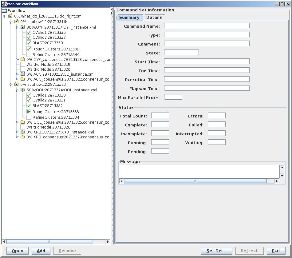
test $ RunWorkflow -t test_run.xml -c test_run.ini -i test_instance.xml &To monitor progress in a GUI environment, make sure you are forwarding X11 packets, then:
test $ MonitorWorkflow -i test_instance.xml &
To monitor progress in your terminal:
test $ ../../WF_monitor.py test_instance.xml 30
 ../../Synergy2-1.1/WF_monitor.py ti.xml
;test ---->running
1.1;subflow1.1 ---->running
1.1;IGQ ---->running
0.333   1       0       3       1.1;IGQ running
1.1;HAY ---->incomplete
1.1;root ---->incomplete
1.2;subflow1.2 ---->running
1.2;XSL ---->running
0.333   1       0       3       1.2;XSL running

running:  3
incomplete:  2


0.333   1       0       3       1.1;IGQ running
0.333   1       0       3       1.2;XSL running

running:  3
incomplete: 2|
|
30 is the number of seconds between refresh |
After the WorkFlow instance has completed, the results need to be translated back to identifiers that correspond to the user-specified data. This can be done for any node, but to get the clustering data for all genomes, it must be done for the root node, which is always test/nodes/root/. Run ClusterPostProcessing.py.
test $ ../../bin/ClusterPostProcessing.py genomes/ nodes/root/locus_mapping.pkl 5
total genes:  24570
pairs: 43456
scc: 3854
mcc: 51
aux: 1280
orphans: 1270
non-orphan clusters: 5185
This will generate several files in nodes/ACC/.
final_clusters.txt - each line of this file describes 1 cluster
clust_to_trans.txt - a 2-column mapping of cluster ID to gene ID
tuple_pairs.pkl - used to calculate the Jaccard Coefficient between two clustering analyses with JaccardPickleComparator.py
summary_stats.txt - used as input for SummaryStatsParse.py
To see if the results you have generated match the results in the example, run the following. It is of note that BLAST is not a deterministic algorithm and your results may differ slightly.
test $ ../../bin/JaccardPickleComparator.py ../results/tuple_pairs.pkl nodes/root/tuple_pairs.pkl
intersecting: 43456.0
all: 43456.0
Jaccard Coefficient: 1.0

test $ ../../SummaryStatsParse.py nodes/root/summary_stats.txt 5
rows: total, valid 6455 5185
score 23984.1441749
avg std dev 6.84571322936
avg std dev/mean length 0.0225223388352